Gradient descent on a Softmax cross-entropy cost function

In this blog post, you will learn how to implement gradient descent on a linear classifier with a Softmax cross-entropy loss function. I recently had to implement this from scratch, during the CS231 course offered by Stanford on visual recognition. Andrej was kind enough to give us the final form of the derived gradient in the course notes, but I couldn’t find anywhere the extended version so I thought that it might be useful to do a step-by-step tutorial for other fellow students. If you’re already familiar with linear classifiers and the Softmax cross-entropy function feel free to skip the next part and go directly to the partial derivatives.

Here is how our linear classifier looks like.

png

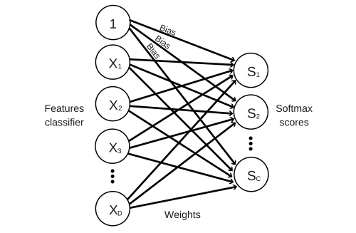
This classifier simply takes the input features $X$ , multiplies them with a matrix of weights $W$ and adds a vector of biases $b$ afterwards. This will give us a score $f_{i}=W_{i}^TX+b_i$ for each $i_{th}$ class in our classifier. We will then pass this score through a Softmax activation function $S_i=\frac{e^{f_{i}}}{\sum_{i=1}^{C}e^{f_{i}}}$ which outputs a value from 0 to 1. This output can be interpreted as a probability (e.g. a score $S_i$ of 0.8 can be interpreted as a 80% probability that the sample belongs to the $i$ class) and the sum of all probabilities will add up to 1.

In order to assess how good or bad are the predictions of our model, we will use the Softmax cross-entropy cost function $L=-log(S_{y})$ which takes the predicted probability for the correct class $S_{y}=\frac{e^{f_{y}}}{\sum_{i=1}^{C}e^{f_{i}}}$ and passes it through the natural logarithm function. If we predict 1 for the correct class and 0 for the rest of the classes (the only possible way to get a 1 on the correct class), the cost function will be really happy with our prediction and give us a loss of 0.

Hopefully, your dataset will have more than one sample so your log loss will be the average log loss on the entire dataset.

As a form of regularization, the L2 norm of the weights is added to the loss function $L=-log(S_{y})+\frac{1}{2}\lambda\sum{W^2}$ ( $\lambda$ controls the strength of the regularization ). This term helps to reduce overfitting our training data and is controlling the magnitudes of our weights.

Here is how you can compute the probabilities and the loss on a toy dataset, in Python.

# Import useful libraries
from sklearn.datasets import make_classification
import matplotlib.pyplot as plt
import numpy as np

# Show plots inline
%matplotlib inline
plt.rcParams['figure.figsize'] = (7,5)

# Generate toy dataset for classification
# X is a matrix of n_samples x n_features and represents the input features
# y is a vector with length n_samples and represents our target
X, y = make_classification(n_samples=1000, n_features=2, n_redundant=0,
                           random_state=2016, n_clusters_per_class=1,
                           n_classes=3)

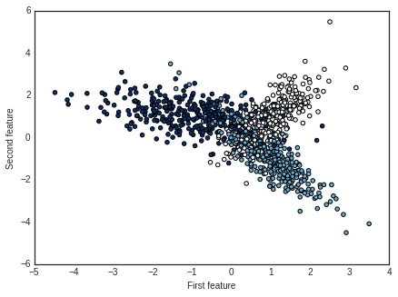
# Visualize generated dataset
plt.style.use('seaborn-white') # change default style of plot
plt.scatter(X[:,0], X[:,1], c=y, cmap=plt.cm.Blues)
plt.xlabel('First feature')
plt.ylabel('Second feature')
plt.show()

png

# Getting some useful parameters
n_features = X.shape[1] # number of features
n_samples = X.shape[0] # number of samples
n_classes = len(np.unique(y)) # number of classes in the dataset

# Initialize weights randomly from a Gaussian distribution
std = 1e-3 # standard deviation of the normal distribution
W = np.random.normal(loc=0.0, scale=std, size=(n_features, n_classes))

# Initialize biases with 0
b = np.zeros(n_classes)

# Linear mapping scores
scores = np.dot(X,W)+b

# Exponential scores
# Normalize the scores beforehand with max as zero to avoid
# numerical problems with the exponential
exp_scores = np.exp(scores - np.max(scores, axis=1, keepdims=True))

# Softmax activation
probs = exp_scores/np.sum(exp_scores, axis=1, keepdims=True)

# Log loss of the correct class of each of our samples
correct_logprobs = -np.log(probs[np.arange(n_samples), y])

# Compute the average loss
loss = np.sum(correct_logprobs)/n_samples

# Add regularization using the L2 norm
# reg is a hyperparameter and controls the strength of regularization
reg = 0.5
reg_loss = 0.5*reg*np.sum(W*W)
loss += reg_loss

Now that we have computed our predictions and loss, we can start minimizing our loss function with gradient descent. For this, we will have to derive the loss function with respect to the weights and bias of each $i_{th}$ class. You can also derive the loss with respect to the input features $X$ but it’s not useful as we are not changing the values of the features when minimizing the cost function.

To compute the derivative of the loss function with respect to its weights $W_{i}$ , we will use the chain rule ${\frac{\partial p}{\partial t}}={\frac{\partial p}{\partial q}} {\frac{\partial q}{\partial t}}$ . This rule is extremely useful for our case, where we have functions nested inside other functions. We can rewrite the loss function as $L = L_{pred} + L_{reg}$ where $L_{pred}$ is our log loss and $L_{reg}$ is our L2 norm of the weights.

$\frac{\partial L}{\partial W_i}=\frac{\partial L_{pred}}{\partial W_i}+\frac{\partial L_{reg}}{\partial W_i}={\frac{\partial L_{pred}}{\partial S_{y}}} {\frac{\partial S_{y}}{\partial f_i}}{\frac{\partial f_i}{\partial W_i}}+\frac{\partial L_{reg}}{\partial W_i}$ ${\frac{\partial L_{reg}}{\partial W_{i}}}={\frac{\partial (\frac{1}{2}\lambda\sum{W^2})}{\partial W_{i}}}={2\frac{1}{2}\lambda W_i}={\lambda W_i}$ ${\frac{\partial L_{pred}}{\partial S_{y}}}={\frac{\partial (-logS_{y})}{\partial S_{y}}}={-\frac{1}{S_{y}}}$ ${\frac{\partial f_i}{\partial W_i}}={\frac{\partial (W_{i}^TX+b_i)}{\partial W_i}} ={X}$

For the $\frac{\partial S_{y}}{\partial f_i}$ derivative, we will use the quotient rule, which states that the derivative of a function $f(x)=\frac{g(x)}{h(x)}$ is equal to $f'(x)=\frac{g'(x)h(x)-h'(x)g(x)}{[h(x)]^2}$ . We also need to distinguish between two cases. The first case is when $i=y$ :

${\frac{\partial S_{y}}{\partial f_i}}=\frac{\partial (\frac{e^{f_{y}}}{\sum_{i=1}^{C}e^{f_{i}}})}{\partial f_i}=\frac{(e^{f_{y}})'\sum_{i=1}^{C}e^{f_{i}} -(\sum_{i=1}^{C}e^{f_{i}})'e^{f_{y}}}{[\sum_{i=1}^{C}e^{f_{i}}]^2}$ $=\frac{e^{f_{y}}\sum_{i=1}^{C}e^{f_{i}}-e^{f_{i}}e^{f_{y}}}{[\sum_{i=1}^{C}e^{f_{i}}]^2} =\frac{e^{f_{y}}}{\sum_{i=1}^{C}e^{f_{i}}}\frac{\sum_{i=1}^{C}e^{f_{i}}-e^{f_{i}}}{\sum_{i=1}^{C}e^{f_{i}}}=S_{y}(1-S_{i})$

When $i \neq y$ , we will have:

${\frac{\partial S_{y}}{\partial f_i}}=\frac{\partial (\frac{e^{f_{y}}}{\sum_{i=1}^{C}e^{f_{i}}})}{\partial f_i}=\frac{(e^{f_{y}})'\sum_{i=1}^{C}e^{f_{i}} -(\sum_{i=1}^{C}e^{f_{i}})'e^{f_{y}}}{[\sum_{i=1}^{C}e^{f_{i}}]^2}$ $=\frac{0\sum_{i=1}^{C}e^{f_{i}}-e^{f_{i}}e^{f_{y}}}{[\sum_{i=1}^{C}e^{f_{i}}]^2} =\frac{-e^{f_{i}}e^{f_{y}}}{[\sum_{i=1}^{C}e^{f_{i}}]^2}=-S_iS_y$

After wrapping it all up, we finally get: $\frac{\partial L}{\partial W_i}=\begin{cases} -\frac{1}{S_y}S_{y}(1-S_{i})X+\lambda W_i & \text{if $i=y$}\newline -\frac{1}{S_y}(-S_iS_y)X+\lambda W_i & \text{if $i \neq y$} \end{cases}=\begin{cases} (S_i-1)X+\lambda W_i & \text{if $i=y$}\newline S_iX+\lambda W_i & \text{if $i \neq y$} \end{cases}$

Similarly, to compute the derivative with respect to the bias we just have to change the last term of the chained derivatives. We can leave out the derivative of the regularization loss with respect to the bias as there is no bias in it.

$\frac{\partial L}{\partial b_i}={\frac{\partial L_{pred}}{\partial S_{y}}} {\frac{\partial S_{y}}{\partial f_i}}{\frac{\partial f_i}{\partial b_i}}$ ${\frac{\partial f_i}{\partial b_i}}={\frac{\partial (W_{i}^TX+b_i)}{\partial b_i}} =1$ $\frac{\partial L}{\partial b_i}=\begin{cases} S_i-1 & \text{if $i=y$}\newline S_i & \text{if $i \neq y$} \end{cases}$

We can compute the gradients on our toy dataset with just a few lines of code.

# Gradient of the loss with respect to scores
dscores = probs.copy()

# Substract 1 from the scores of the correct class
dscores[np.arange(n_samples),y] -= 1

# Instead of dividing both dW and db with the number of
# samples it's easier to divide dscores beforehand
dscores /= n_samples

# Gradient of the loss with respect to weights
dW = X.T.dot(dscores) 

# Add gradient regularization 
dW += reg*W

# Gradient of the loss with respect to biases
db = np.sum(dscores, axis=0, keepdims=True)

At this point, we have everything we need to start training our model with gradient descent. We’ll use a simple updating rule, with only one hyperparameter $\alpha$ which controls the step size of the update. There are more advanced updating techniques like Nesterov momentum or Adam which I definitely recommend you to try out.

$W_i=W_i-\alpha\frac{\partial L}{\partial W_i}$ $b_i=b_i-\alpha\frac{\partial L}{\partial b_i}$

Since gradient descent is an iterative method, we also have to set manually the number of iterations. This can be tricky as a suboptimal number of iterations can lead to either underfitting or overfitting the model. Instead of choosing the number of iterations manually, we can split the data into a training and validation set and use early stopping on our validation samples to avoid overfitting our model on the training set. The validation set can also be used to tune your hyperparameters $\alpha$ and $\lambda$ .

I have created a class for the Softmax linear classifier, based on the first assignment of CS231. You can find it here.

You can use this class either to train your entire dataset with softmax.train() or you can use softmax.train_early_stopping() to stop training if there is no improvement in the accuracy of your predictions on the validation dataset, after a certain number of iterations.

# Split dataset into training and validation
X_train, y_train = X[0:800], y[0:800]
X_val, y_val = X[800:], y[800:]

# Train with early stopping
softmax = Softmax()
softmax.train_early_stopping( X_train, y_train, X_val, y_val,
                             learning_rate=1e-2, reg=0.1,
                             early_stopping_rounds=300)
print('Training accuracy',np.mean(softmax.predict(X_train)==y_train))
print('Validation accuracy',np.mean(softmax.predict(X_val)==y_val))

Training accuracy 0.815
Validation accuracy 0.805

# Train on the entire dataset
softmax = Softmax()
softmax.train(X, y, learning_rate=1e-2, reg=0.1, num_iters=1000)
print('Training accuracy', np.mean(softmax.predict(X)==y))

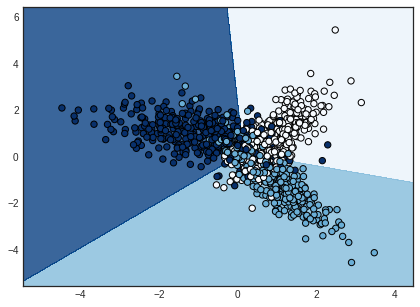
Training accuracy 0.816

These are our decision boundaries after training on the entire dataset.

# Create a mesh to plot in
x_min, x_max = X[:, 0].min() - 1, X[:, 0].max() + 1
y_min, y_max = X[:, 1].min() - 1, X[:, 1].max() + 1
xx, yy = np.meshgrid(np.arange(x_min, x_max, 0.01),
                     np.arange(y_min, y_max, 0.01))

# Predict target for each sample xx, yy
Z = softmax.predict(np.c_[xx.ravel(), yy.ravel()])

# Put the result into a color plot
Z = Z.reshape(xx.shape)
fig = plt.figure()
plt.contourf(xx, yy, Z, cmap=plt.cm.Blues, alpha=0.8)

# Plot our training points
plt.scatter(X[:, 0], X[:, 1], c=y, s=40, cmap=plt.cm.Blues)
plt.xlim(xx.min(), xx.max())
plt.ylim(yy.min(), yy.max())
plt.show()

png

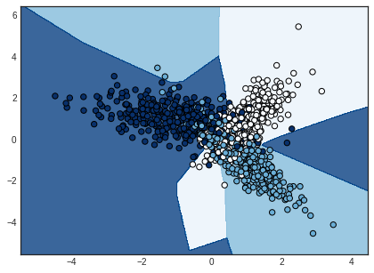
Looking for more ‘exotic’ decision boundaries? Try a neural network. This is what I get with a single hidden layer neural network trained with the same cross-entropy loss function. Though it’s a perfect example of overfitting your training data.

png

I hope that you found this blog post helpful and let me know in the comments below if you have any questions.